On Sunday 25th February 2024 a small team consisting of members of CAGG and the CVAHS met at Seer Green in Buckinghamshire to explore a site that was seen in the lidar data collected by the Chilterns Conservation Board’s Beacons of the Past project (Fig 1). The lidar indicated quite clearly the presence of a quadrilateral enclosure. On site, the outline of the enclosure could be seen quite clearly through the grass.
Figure 1: local relief model derived from the lidar data of the site. Image derived from lidar collected for the Chilterns Conservation Board to whom thanks are due.
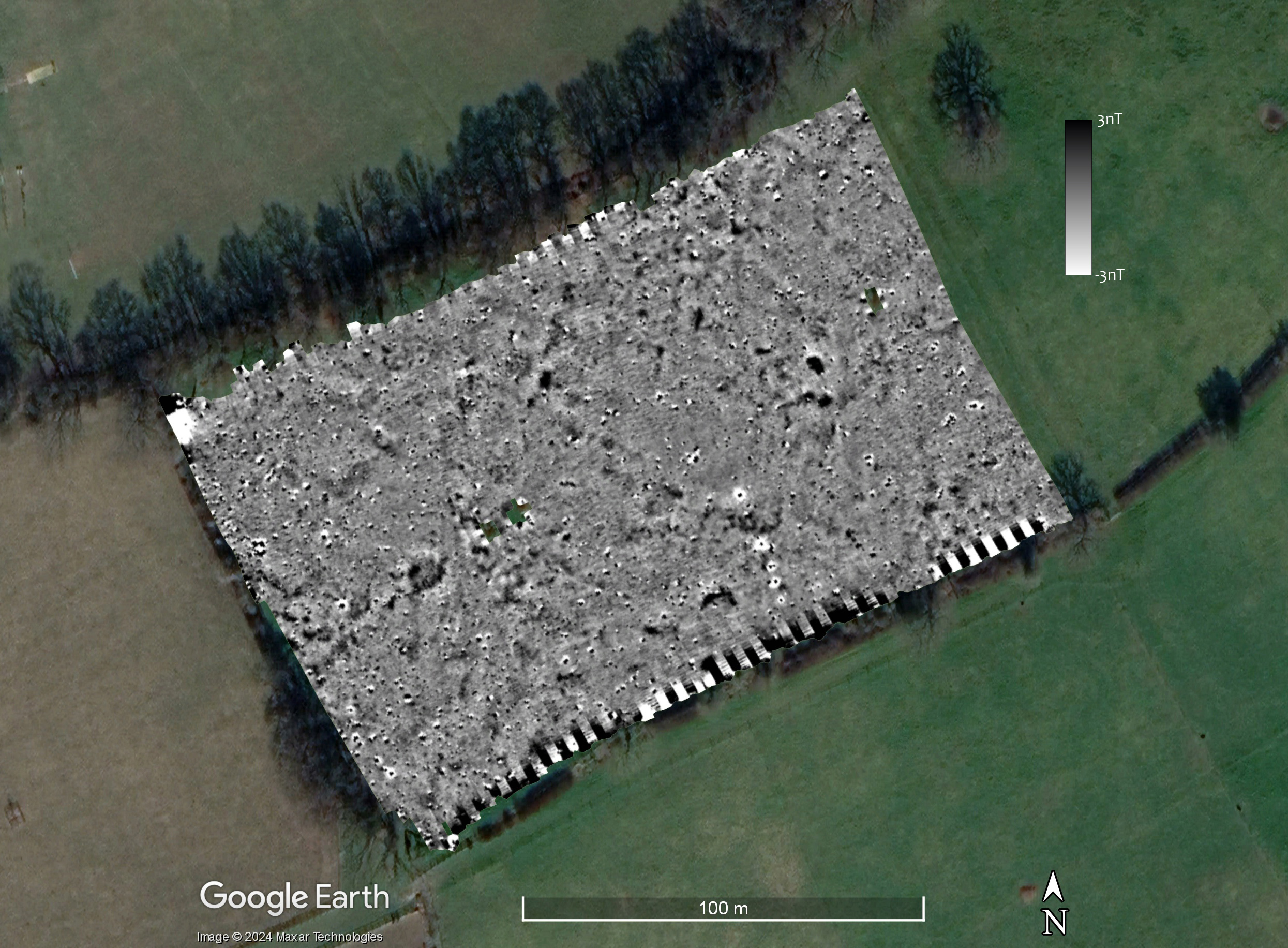
The enclosure can also be seen in the March 2022 imagery available from Google Earth (Fig. 2).
Figure 2: image from Google Earth showing the enclosure.
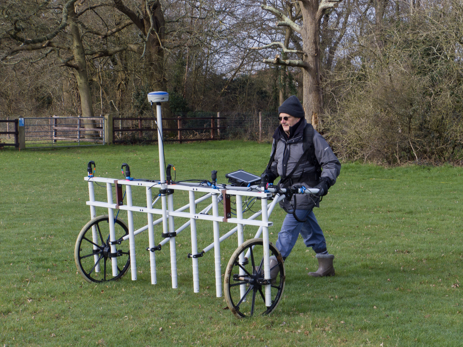
Although it was pretty chilly the ground conditions were good with short grass and not too much mud (Fig. 3) so we were able to complete the whole field in a day, some 2.4ha.
Figure 3: Nigel Rothwell (CVAHS) operates the Sensys magnetometer.
After supper Jim West and I processed the data with high expectations. They were somewhat dashed (Fig. 4).
Figure 4: the magnetometry results.
As can be seen from Figure 4, the enclosure does not show in the mag results at all. This is very disappointing. We should keep in mind, however, any geophysical survey technique does not always detect subsurface features: there has to be some contrast in the property being measured. A good example is the colonnaded “palace” building at Verulamium which does not show in the mag at all but shows in the GPR data very clearly.
In Figure 5 I have added a crude outline of the “enclosure” created by simply drawing a line around the vegetation marks in the Google Earth image. Although the large “ditch” does not show, there are some features in the mag data. I have indicated one with the red arrow.
Figure 5: the mag survey with the outline of the “enclosure” and one of the possible features indicated.
So although we didn’t detect the enclosure ditch, there are some features in the data. I have indicated just one with a red arrow in Figure 5. This is a roughly rectangular feature about 5m long and 2.5m wide. Just on its southern edge is a smaller “dot” of high readings with a corresponding low magnetic reading. In Figure 6 I have taken a screen shot from TerraSurveyor where I have drawn line across the feature and obtained the readings as a graph (Figure 6).
Figure 6: Screenshot from TerraSurveyor showing the readings across a feature in the survey.
In Figure 6 I have divided the graph into two zones. The rectangular feature has nanotesla values of between -2 and +6. The asymmetrical values are typical of an archaeological feature which is, in part at least, derived from magnetic susceptibility. As a result of the Earth’s magnetic field, features which show because of mag sus will have their main area of negative magnetism to the north. The smaller “dot” feature, however, has a range of c. -6 to +8 nT. Although these are not especially high values. they are more evenly balanced and the area of the negative values is similar to the positive. It is likely, therefore, that the “dot” is a result of something ferrous, although probably something quite small.
There are, therefore, a scatter of probable and possible archaeological features. How could we be sure? Some form of “ground truthing” would be needed. This could be digging a test pit, or could be simply putting a small auger into the features and around them.
Why the large ditch (if that is what it is) does not show is more problematic. The fill of the ditch is not more magnetic than the surrounding soils. Perhaps the bank was deliberately backfilled into the ditch and thus mainly putting the subsoil back into the hole it came from? This is just a guess. We should also note that the site was wooded from the mid-16th to the mid-19th centuries. The removal of mature trees may have had an impact. The geology here is Beaconsfield gravels. These are described by the British Geological Society as comprising “1 – 7 m of variably sandy and clayey gravel”. Perhaps these gravels are not good for magnetometry? I would have liked to take some mag sus readings at the site as we have elsewhere. I’m slowly building-up a databank of readings which, eventually, I can compare to the geology and the “success” of the mag surveys. What I do know is that we seem to have rather poor results for surveys we have undertaken for CVAHS!
The survey was undertaken by Jim West, Janet Rothwell, Nigel Rothwell and Kris Lockyear. The equipment was provided by the Institute of Archaeology, UCL. Many thanks to the landowner, Sir Andrew Witty and and to Julian Faircloth who facilitated our access.
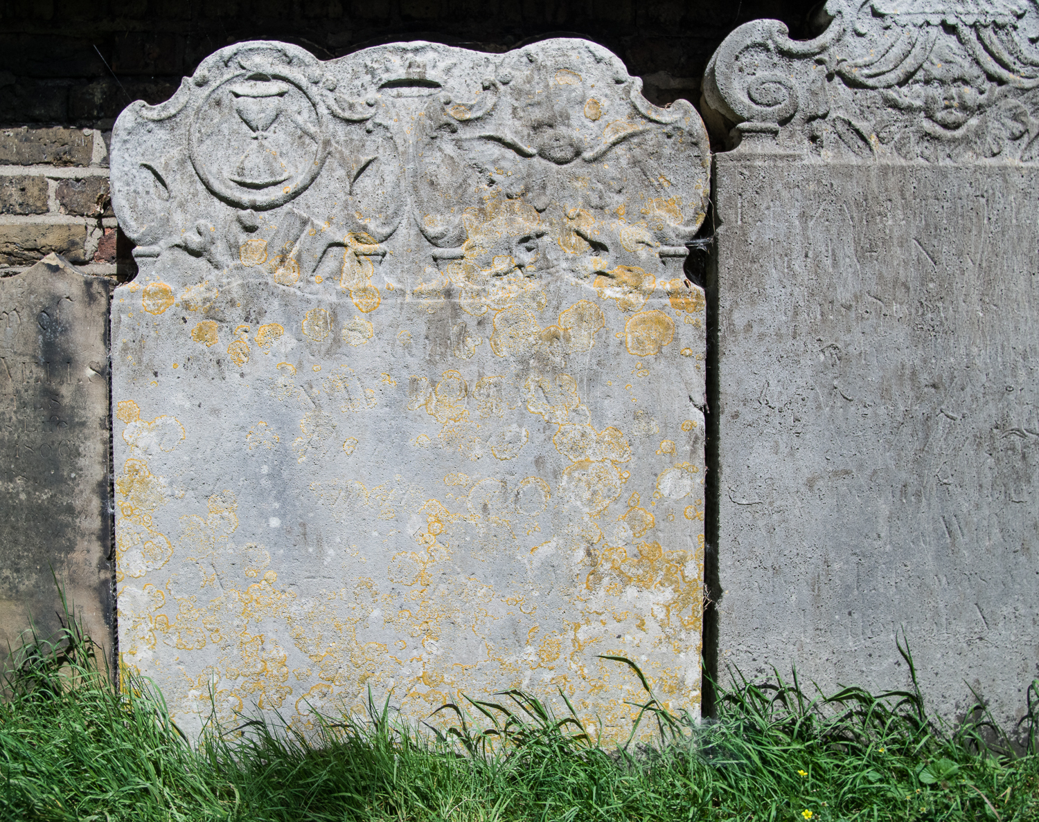
Last year I was asked by Ken Walton from the Institute of Archaeology, on behalf of Chris Baker (Director of Dartford District Archaeological Group) and Dr Mike Still (Curator of Dartford Borough Museum), if we would be willing to undertake some survey in Dartford, specifically in “St Edmunds Pleasance”, a small disused cemetery which is used now as a park. Sadly, the majority of the headstones — including some lovely eighteenth century examples with memento mori (Fig. 1) — have been moved and are now around the edges of the area.
Figure 1: tombstone with memento mori. Note the hourglass reminding us of the passage of time and the two skulls reminding us of our mortality.
The larger chest tombs have been left in place (Fig. 2). The cemetery also has a monument to the Dartford martyrs (Fig. 3). This monument was built in 1851 in memory of three protestants, Christopher Ward, Nicholas Hall and Margery Pollen, who were burnt at Dartford in 1555. The monument is listed.
Figure 2: chest tomb to John Hall who died in 1836. John Hall was Richard Trevithick’s last employer.Figure 3: monument to the Dartford martyrs built in 1851.
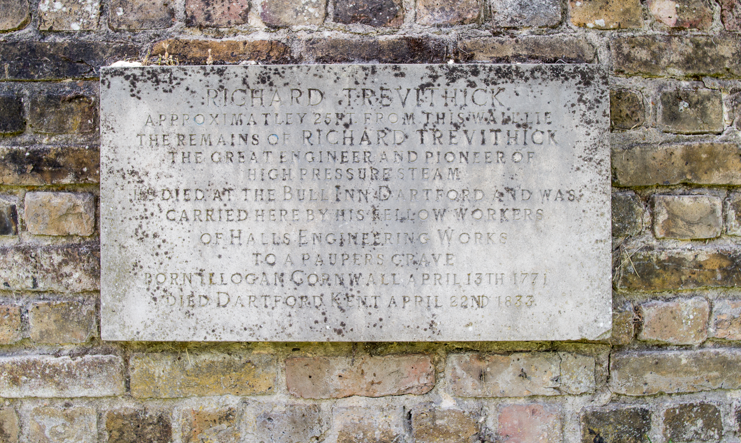
Perhaps the most interesting aspect of this cemetery, however, is that it is the final resting place of Richard Trevithick. Trevithick was a Cornish engineer and inventor. He designed and built a number of high-pressure steam engines. One of those, the Catch-me-who-can ran on a circular track just south of Euston, now identified as being located on the site of the Chadwick building at UCL. Trevithick died a pauper in Dartford in 1833 and was buried here in a pauper’s grave (Fig. 4).
Figure 4: plaque commemorating the burial of Richard Trevithick at Dartford.
So, what has all this to do with geophysics? Apparently, Trevithick’s colleagues who buried him were afraid of body snatchers:
It is interesting to learn of the special steps which were taken in those days to defeat the body snatchers. Thomas Aldous, who was at the works from 1843 to 1879, told the author that his father who was one of Hill’s workmen at the funeral. He described the coffin as being fitted with two long stout pieces of timber placed at right angles to the coffin above and two pieces below: these were strongly bolted together so as to clamp the coffin between them, and as a further precaution the nuts of the bolts were under the bottom timbers so they could not be disturbed from above. It is obvious that to get the body out the who structure must be removed necessitating the excavation of an enormous hole.
Evarard Hesketh (1935). J. and E. Hall Ltd 1785-1935, p.14.
My worry about this story is that it sounds a little at odds with “a pauper’s grave”, although Trevithick died only five years after the infamous case of Burke and Hare which may lend it more credence. If true, however, there should be at least four vertical iron bolts. Iron objects on end have a distinctive signature in magnetometry data. They usually have a strong positive reading as a small point and then a “halo” of negative readings around them. It was a very long shot, but it was worth a day trip to Dartford, so in July last year (2022), Jim, Ruth and I headed to the cemetery to undertake a day’s survey.
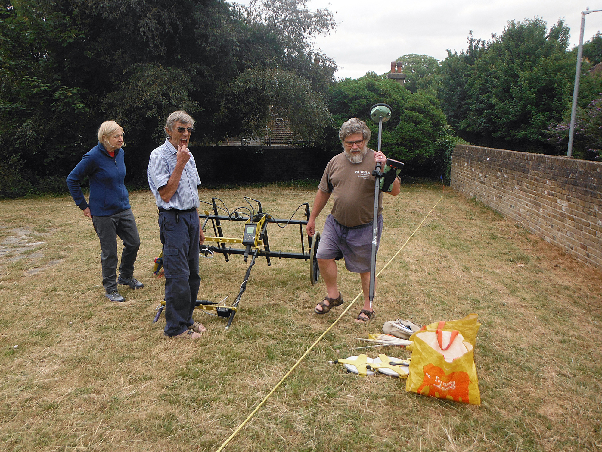
The survey took place when we were using the Foerster magnetometer. This meant that we had to lay out a rather complex set of grids and indulge in quite a bit of wheel spinning. This made the survey slow given the head scratching involved, not helped by the many trees which blocked the GPS signal (Figs. 5 and 6).
Figure 5: Ruth, Jim and Kris map out the grids of the survey. Photo: Ken Walton.Figure 6: Jim West using the Foerster magnetometer. Photo: Ken Walton.
We managed to survey three areas: one near the plaque on the wall, one near a second entrance which might be where Trevithick was buried, and a third out of interest due to some parch marks in the grass (Fig. 7).
Figure 7: the three mag areas.
In area one there are a number of ferrous items: two bins on steel bases and an area of fencing along the wall, as well as two paths, one a decorative sinuous path of crazy paving and the other a tarmac path (Fig. 8).
Figure 8: view across area 1 showing the fencing, bins and sinuous path.
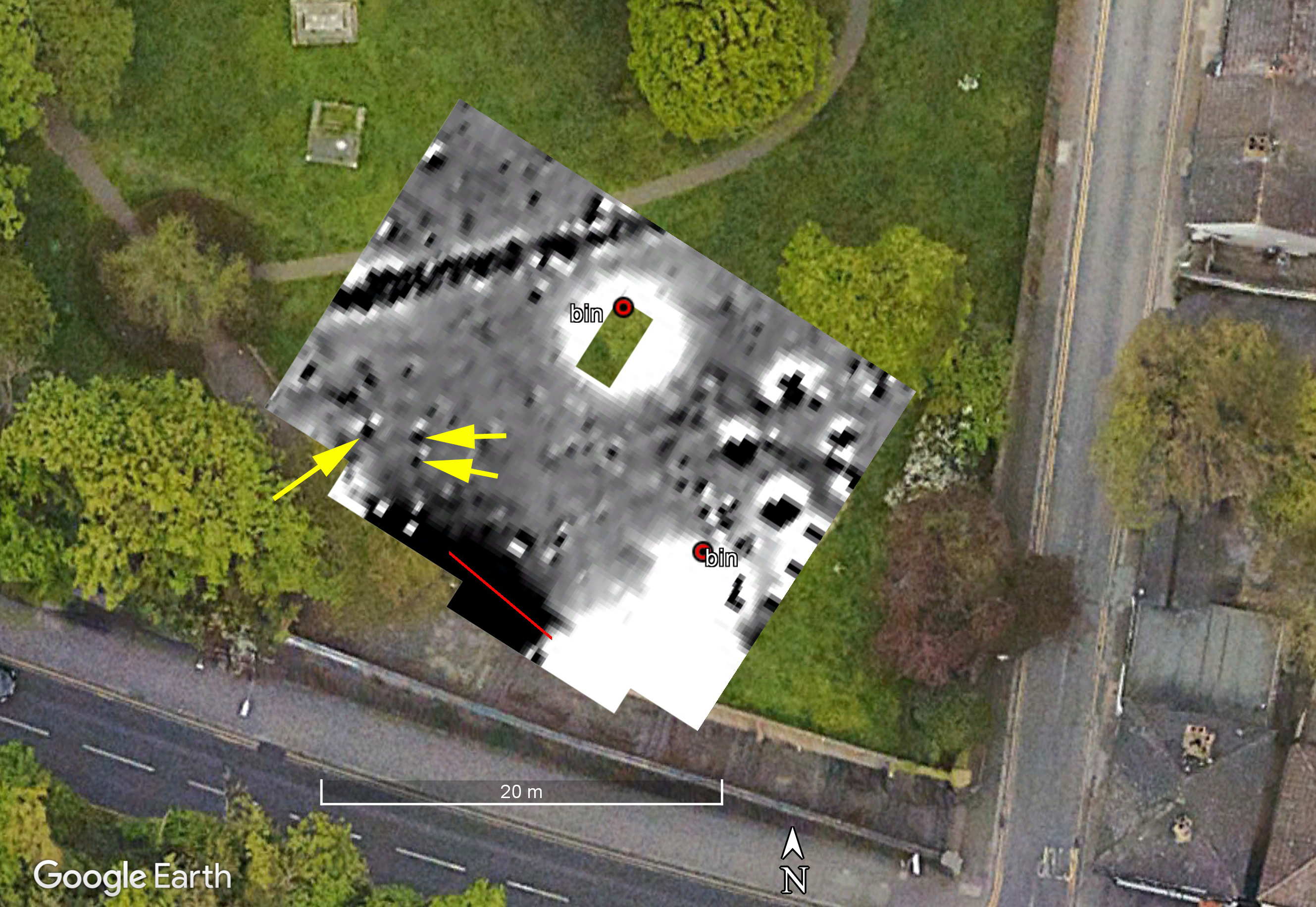
The mag results are shown in Figure 9. For reasons I haven’t managed to sort out, the survey is about 2m further south on the Google Earth image than it should be. As can been seen, the dark line representing the tarmac path in the mag data does not quite line-up with the actual path. I’ve marked the two bins, and the red line represents the railings. Significant areas of the survey are masked by strong ferrous responses like the bin and the fence. There are also some big ferrous objects in the eastern half of the survey. There are, however, some weaker features. I have marked three with yellow arrows. East-west they are 2.5m apart and north-south 1.5m. Are these Trevithick? I think I am grasping at straws but I guess it is possible, although perhaps unlikely.
Figure 9: The mag results from Area 1. The red line presents the iron fence seen in Figure 8.
Area 2 was chosen as it is near the second entrance to the cemetery and some of the sources can be interpreted as saying Trevithick was buried there. The large number of trees made surveying in the grid very difficult, and again the mag is not quite in the right place (Fig. 10). We can see, however, that really the only thing that shows is the iron work on the western edge of the area, and the two paths which cut across it.
Figure 10: the magnetometry results from Area 2.
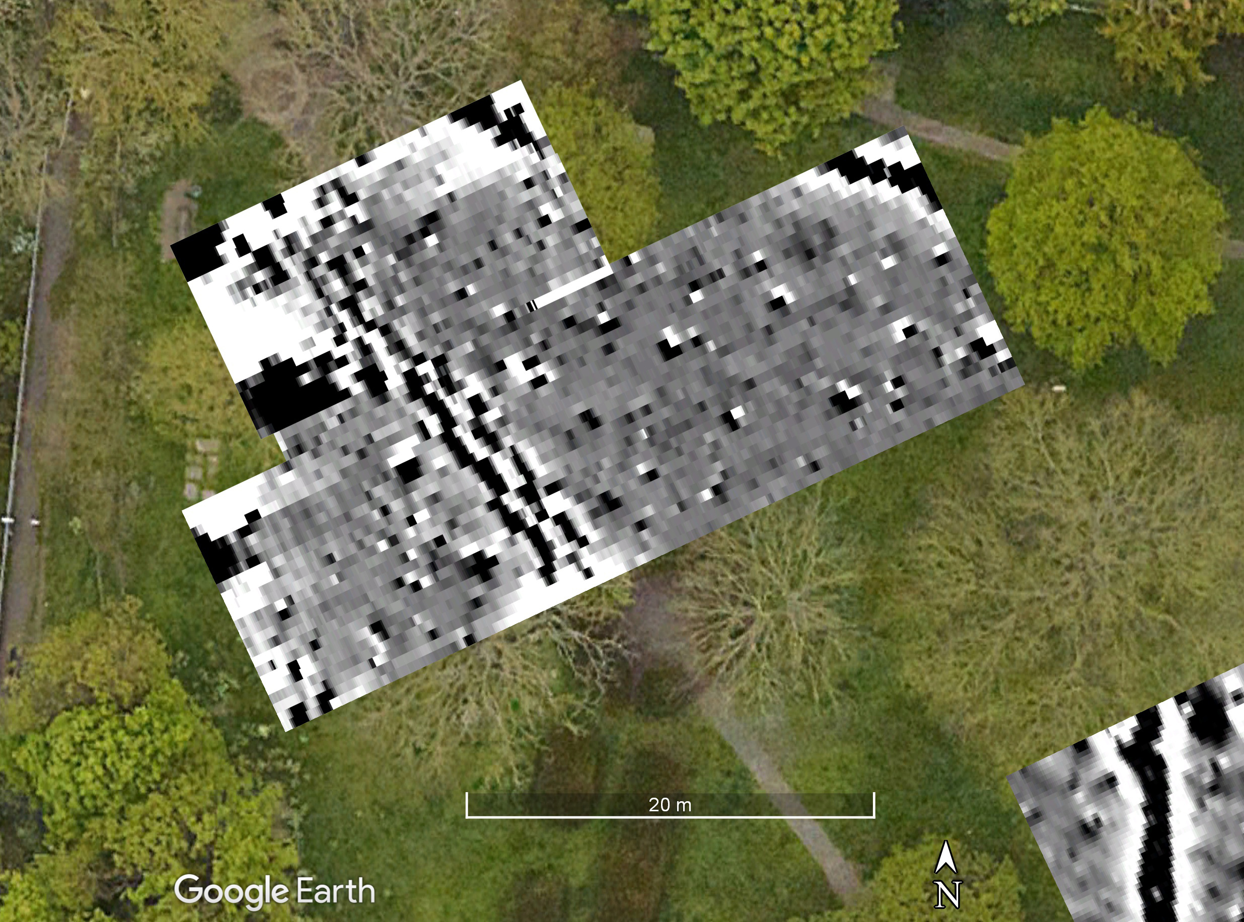
Area 3 was chosen for different reasons. It lies in a relatively open area of the cemetery, and had some interesting looking parch marks. There had been a chapel but this had largely gone by the 18th century and we are unsure, exactly, where the chapel lies. We were hoping the parch marks might show us the location of the chapel. It was, thankfully, a relatively straightforward block of mag data to collect at the end of our day (Fig. 11).
Figure 11: Mag results from Area 3. See text.
In Figure 11 the linear feature marked with yellow arrows is the classic signature for an iron service pipe, either water or gas probably. The fact it heads directly towards the gate in the eastern wall is not a surprise. The dark line indicated with the light blue arrows looks like other paths we have seen in the park, but this one is clearly completely over-grown. Finally, there is the curious circular feature in the middle of the plot. Aerial photographs in Dartford Museum from 1960 and 1971 show that there was a ornamental feature here. The 1960 photograph also clearly shows the path we have mapped. The 1960 photo shows that the tombstones had been moved by that date and that the park was well-tended with circular flower beds.
Although the mag results were not very exciting, the prospect of finding the “missing” chapel drew Mike Smith and I back to Dartford in August 2023 with the GPR. The new GPS that is normally on our Sensys magnetometer freed us from having to work in traditional grids, and has fewer problems with the tree cover (Fig. 12).
Figure 12: Kris (wearing the same Welwyn Archaeological Society tee-shirt as in Fig. 5!) pushing the GPR in Area 1 with the new GPS attached.
We surveyed two area: one roughly coincident with Area 1 and a second in the hopes of locating the chapel in Area 2. The advantage of using the dGPS is that it saves on laying out grids, and you get a cool map of where you have been (fig. 13)!
Figure 13: Timeslice 5 (10.5 to 12.5 ns) with the GPS tracks overlaid.
The GPR survey in Area 1 picked-up the tarmac path and the crazy-paving horse-shoe shaped path, but very little else. Figure 14 shows timeslice 5 (10.5 to 12.5ns) and Figure 15 shows slices 2 to 10.
Figure 14: time slice 5 (10.5 to 12.5 ns).Figure 15: Timeslices 2 to 10.
I was very surprised at how little was showing and how persistent the surface features are. I very much doubt that the crazy-paving path was more than a few inches thick, and yet it persists in the slices down through the sequence. Looking at the amplitude profile (aka ‘radargram’) we can see that we are getting very little real depth penetration (only to about 15ns). The horizontal banding that can be seen in Figure 16 is typical of radargrams before they have had a “background removal” routine performed on them. This image, however, is of a radargram after background removal!
Figure 16: Profile 28. The strong flat reflections are the paths.
This suggests we have not got a very deep penetration and almost everything we are seeing is either at the surface or just below. I’m investigating why as conditions should have been OK on this site.
The second survey which overlapped with Area 3 of the mag survey showed some interesting features. Figure 17 shows the third time slice (5.9 to 9.4ns, 0.3-0.5m below surface). The double-circle is the garden feature which shows in the 1960 photograph with a path coming off to the west. This path joins the one shown by the light blue arrows in Figure 11 and can also be seen in the photo. The discontinuous nature of the circle on the northern side is probably because the service shown with yellow arrows in Figure 11 cuts through the circle at this point.
Figure 17: Area 3 GPR survey. Timeslice from 5.9 to 9.4ns, 0.3-0.5m below surface.
Looking slightly deeper there is quite a strong reflection marked in Figure 18 with a yellow arrow. This corresponds to an area of ferrous noise seen in Figure 11 marked with a red arrow.
Figure 18: GPR slice 5 (11.9 to 15.4ns, 0.6 to 0.8m below surface).
This big feature shows clearly in the radargrams (Fig. 19, red arrow).
Figure 19: Profile 107 with the large feature indicated with the red arrow.
Given the size of the feature, its orientation and the complex reflections shown in the profile, I suspect this may be a burial vault which would have lain under a monument like that shown in Figure 2. Compare the size and shape of it to the one which can be seen near to the road in Figure 18. Some of the other “blobs” (technical term that!) may be similar things. There is also a faint hint of the service in Figure 18 as shown by the blue arrows.
Despite our best efforts both Trevithick’s grave and the chapel eluded us. But we had two pleasant days none-the-less. Thanks to Ruth, Jim and Mike for their hard work, and to Ken Walton, Chris Baker and Mike Still for setting this up, to the Dartford District Archaeological Group for hosting us and the Forrester’s pub for letting us use their car park and a nice pint of real ale at the end of the day (Figure 20)! Many thanks also to Dartford Borough Council for allowing us to undertake these surveys. Perhaps next year we could try res…
The Leighton Buzzard and District Archaeological and Historical Society (LBDAHS) having been trying to locate the “Holy Well” at Linslade since 2018. The well was very popular in the medieval period, especially in the 13th century. The waters reputedly had healing properties. The well is marked on old maps such as the first edition OS map, but the accuracy of the location is uncertain. The Society have managed to locate a small cottage of 18th or early 19th century date on the banks of the canal which they have partially excavated (Figure 1). In 1915 local historian J. G. Gurney mentioned an old cottage and garden that lay “on the exact site of the Holy Well”, and included a sketch map. This is certainly the cottage which is being excavated.
Figure 1: the post-medieval cottage excavation.
As well as a variety of post-medieval finds, some of the features have included some sherds of medieval pottery of the right date, and one trench a little to the north of the cottage contained a Romano-British pottery sherd.
From a geophysics point of view the site is quite difficult. The main area of interest is the strip along the edge of the canal which has thick riverside vegetation. The excavation trenches regularly fill with water. The site is, however, on the edge of a steep slope down the canal and so gets drier quite quickly as one moves upslope. What were we hoping to find? One suggestion was that because the well was so popular there might be some form of path or track to the well. If we could detect that, perhaps this would give a clue as to its location.
Pauline, stalwart member of both LBDAHS and CAGG, arranged for us to undertake an exploratory Earth Resistance survey at the site. Due to covid and other commitments this took a bit of time to organise, but finally we managed to earmark a couple of days on site (Fig. 2).
Figure 2: the Earth Resistance survey underway.
The survey was somewhat jinxed! On the first day, we couldn’t get a reading at all to begin with. I spent quite some time checking the cables and connections and generally making sure all seemed OK to no avail. In desperation I reset the machine to its “factory” defaults and hey presto, all started to work again. Then, as we were working, one of the welds on the frame broke. Luckily we could keep on working by holding the frame on the sides, and the next day a temporary repair was effected by the liberal use of duck tape. On the second morning I found that we had dropped a bracket from the GPS the day before when packing-up. Thankfully, using the GPS to locate where we packed-up and some careful searching around that point, we managed to find it again. Phew.
On the first day, Pauline, Rhian, Kate and I surveyed a line of grid squares parallel to the canal. Partly due to the vegetation we did not get too close to the canal. Also, the waterlogging would result in featureless results and so it simply was not worth the effort (Fig. 3).
Figure 3: Rhian using the Geoscan RM85 Earth Resistance meter.
On the second day we surveyed a block of grids closer to the current road to see if we could pick-up any buildings in that area. As we usually do, we used the 1+2 method. The RM85’s built-in multiplexer (basically a fancy switching box) means that we collect three readings with each movement of the frame. The first reading has a 1m probe separation and the second two have a 0.5m separation. The 1m separation looks about a meter or so into the ground and the 0.5m separation roughly 0.5–0.7m into the ground. The deeper survey, however, has half the resolution of the shallower survey (1m transect spacing and a 0.5, sample spacing compared to a 0.5m transect spacing and a 0.5m sample spacing).
Figure 4 shows the results of the shallower survey, and Figure 5 the deeper survey.
Figure 4: the 0.5m probe spacing Earth Resistance survey. Black is high resistance.Figure 5: the 1m probe separation Earth Resistance survey.
Looking at Figure 5 first, I would argue that most of what we can see here is geology rather than archaeology. The ground slopes from the bottom of the image to the canal at the top. We can see in the strip of survey at the top of image a band of low resistance readings parallel with the canal. This is almost certainly the transition from the more solid bedrock to river/canal-side deposits and the presence of water. In the area near the road, the high resistance areas near the building are again related to topography rather than archaeology.
The 0.5m probe separation survey in Figure 4 has a few potential features. I have labelled these in Figure 6.
Figure 6: the 0.5m survey labelled.
There is a faint higher resistance line running towards the excavated area on the canalside. This could be a path?
A small rectangular high resistance feature might be the foundation for something.
The blue lines indicate two low-resistance linear features. These might be some sort of cut feature (pipeline, robbed wall lines?).
A high resistance vaguely linear feature.
I wish I could be much more positive with these results and I am the first to admit that none of them are 100% convincing. It might be worth “ground truthing” my tentative interpretations a little more.
Lastly, a thank you to Mike who has subsequently rewelded the frame, and to Jim for making-up some new jump leads ready for the res meter’s next outing.
On Friday 29th November 2019, Kris Lockyear will be giving a talk on the results of the survey work entitled “Verulamium: busy places and empty spaces.” The meeting will start at 7.45pm, United Reformed Church hall, Church Road, Welwyn Garden City. WAS members free, visitors £3.
Anyone new to this blog or geophysics in archaeology is recommended to read the material on the “Geophysical survey in archaeology” page.
One what, I hear you say? Well, 1km2. What is 1km2? Well, that is the area covered by the mag in all the Verulamium-related surveys. Yup, one whole square kilometer. Impressive, eh? By the way, that is about 20,000,000 individual mag readings. That doesn’t include, of course, squares that had to be re-done due to sensor freezes or areas blanked out where we were wheel spinning for partial grids. Congratulations to all who have pushed that machine since the summer of 2013.
Figure 1: Jim West and the mag.
Today the mag team completed the far end of Church Meadow (Figure 2). It is great to see such a huge proportion of the field done, and much of what is left is not worth doing as it is featureless alluvium.
Figure 2: the Church Meadow mag at the end of the 2019 summer season.
Figure 3 shows the details of the southern end of the survey.
Figure 3: Detail of the southern end of the Church Meadow mag survey.
Most of the new area today was either in the area impacted by the pipes, or featureless alluvium. The little partial near the road, however, found a small feature which looks like a wall with something in the middle. Given this is right next to the gate of the town, perhaps this is a mausoleum? No real way of knowing without digging it, but certainly a possibility.
The Earth Resistance team of Debbie, Tim, Denley and Ellen were on form today and completed a super nine grid, thus satisfying my need for a tidy end to a season! Figure 4 shows the results from today.
Figure 4: the Earth Resistance data after day 3.
Figure 5: the Earth Resistance data high-pass filtered.
As can be seen, there are a number of wall showing clearly as dark (high resistance) lines. The room which shows most clearly is the one which can be seen on the Google Earth image. A high-pass filter shows the walls even more clearly (Figure 5).
The GPR crew, allowed down from the heights of the Theatre field, picked a 40×80 strip east-west across the middle of the buildings. Figure 6 shows the first twelve time slices.
Figure 6: GPR time slices across the nunnery.
As can be seen, the building that shows well on Google Earth is visible right from the first time slice. The stone work must be literally just under the surface. Slices 7 and 8 shows the buildings in great detail as well as that pipeline running across the plot. Figure 7 shows slice 7 on the Google Earth image.
Figure 7: GPR data across the nunnery. Slice 7.
To close out the 2019 season posts, I asked Mike Smith to take a group photograph. Not everyone who was involved this summer was there today, but Figure 8 shows a good number of us.
Many, many thanks to everyone who turned-out over the last four weeks, be it almost every day or for just an afternoon. Without the CAGG team members, this project wouldn’t achieve anything! Also, big thanks to Strutt and Parker and the Gorhambury Estate for facilitating access, and to Lord Verulam and his family for all their support. Lastly, thanks to the AHRC for funding the original project back in 2013, the Institute of Archaeology, UCL for supporting the project and the loan of the GPS and the Earth Resistance meter, and to SEAHA for the loan of the GPR.
I’m off to Sligo tomorrow morning at about 4.30am and will be presenting some of our results to the International Conference on Archaeological Prospection on Wednesday afternoon.
Anyone new to this blog or geophysics in archaeology is recommended to read the material on the “Geophysical survey in archaeology” page.
I think Mike Smith would argue that he is “done” in more ways than one! I feel that a suitably sonorous 1950s newscaster voice ought to be saying “at 1pm this afternoon, members of…” The reason? Because at 1pm this afternoon the GPR survey finally surveyed the last part of the theatre field (Figure 1).
Figure 1: Mike Smith crosses the finish line.
That is some 27ha of GPR survey, mostly at 50cm transect spacing. That works out to pushing the mag some 540km across the field. Figure 2 shows the final coverage. As always, the image is a mess because it has been created by different pieces of software at different times and even with slightly different conversions of OS coordinates to lat and long. My big job now is to turn that pig’s ear (processing-wise) into a clear image.
Figure 2: Done. The complete GPR survey of the theatre field (but needs better processing).
Many members of CAGG have contributed to the GPR survey over the last five seasons. This season Nigel Harper-Scott, John Ridge and John Dent have contributed greatly (Figure 3). The person who really deserves a rest, however, is Mike Smith who has not only led the GPR team over most of the last five seasons, but has also been the main GPR transporter during the season, and has been looking after it during the week. Many thanks Mike, and well done on a great achievement.
Figure 3: Nigel (left), Mike (centre) and John (right), today’s GPR crew.
The area covered this year is best seen via the stripes in the grass (Figure 4).
Figure 4: Stripy grass left by the GPR.
Now, you would have thought that completing the survey would have persuaded the boss to let them go home early. Nope. None of that slacking. One grid we did at 1m transect intervals had an interesting building in it. So after lunch the team set to once again to resurvey it at 0.5m intervals. In figure 5 I have made the high amplitude reflections white so that the building can be seen more easily and placed it on the mag survey for context. It is a long, thin, building with a corridor just visible on the eastern side and a larger group of rooms to the south.
Figure 5: the re-done block on the mag data.
Tomorrow, Mike gets his pick of which two squares to survey in Church Meadow.
The mag team re-did all the dodgy squares from yesterday, and quite a few more (Figure 6)!
Figure 6: the mag data in Church Meadow after day 5.
The mag team have just three whole squares for tomorrow, and then a few partials at the ends. For most of its length, it is not going to be worth surveying up to the edge of the field to the NE as it is clearly into alluvium as shown by the flat, featureless mag data. Figure 7 shows a close-up of the southern end of the survey.
Figure 7: the Church Meadow mag data, southern end details.
The darker curvy line is possibly an old edge to the river. There are quite a few small dark blobs (“positive magnetic anomalies”) some of which could be graves, and at least part of a ditch feature. I am still puzzled by the long negative linear. I guess I’ll have to talk to some other geophysicists!
The res team was joined by Denley Lane of the Arc and Arc, Denley remembers some of the pipelines being built. The team completed an excellent seven grid squares. Figure 8 shows the results, and Figure 9 shows the same results high-pass filtered.
Figure 8: the res results in Church Meadow after day 2.
Figure 9: the res results in Church Meadow after day 2, high pass filtered.
As can be seen, the building visible in the Google Earth image shows very well indeed, but there does not seem to be many more buildings to the south. Tomorrow we will fill-in the one last block in the eastern corner, and then do a strip of blocks along the northern edge.
Tomorrow is the last day of the 2019 season. I’ll be speaking about the Project at the International Conference on Archaeological Prospection on Wednesday. Not much time to fit in the new results!
Anyone new to this blog or geophysics in archaeology is recommended to read the material on the “Geophysical survey in archaeology” page.
It was a very warm and sunny day today, and I think we all felt the heat. We managed to complete quite a bit of work, though, and so congratulations to all the team.
The GPR team filled-in some of the missing bits on the west, north and east sides of the theatre field (Figure 1). Just a few bits left now.
Figure 1: The almost-complete GPR survey.
One nice feature was a little detail found on the western side (Figure 2).
Figure 2: A detail of the GPR survey from today. The red arrow indicates a small building.
A nice little building is showing-up. The block to the east may show some robbed buildings. Last year I noticed some curious white lines in that block which could be robbed walls.
The mag team completed an excellent eight grids taking their total area surveyed in four days to 5.09ha. Frustratingly, however, I found that the sensors had frozen on the first three grid squares. Horrible waste of time, but nothing to be done about it. Figure 3 shows the whole survey.
Figure 3: the mag survey in Church Meadow after day 4.
Despite the frozen sensor, we can see some interesting details in the new area to the south (Figure 4).
Figure 4: the southern area of the mag survey in Church Meadow after day 4.
What I am finding curious is that the long linear features are white in the plots, i.e., below average magnetism. The features look like ditches in form, but do not give the usually positive response one would expect from them. My worry is land drains… but the features seem to connect with the edges of Watling Street. How very curious.
Figure 5 shows the Earth Resistance survey after day 1. The team completed an excellent eight grids.
Figure 5: the res survey in Church Meadow after day 1.
The broad dark line across the western corner is Watling Street. Further east the various thinner dark lines are the walls of buildings. Clearly we have parts of a number of structures showing clearly. Great stuff. We don’t have a cruciform-shaped building face east-west yet, but give us time. Hopefully, tomorrow, we will cover the building which shows so clearly in the Google Earth image. Comparing the mag and the res shows how much the pipes obscure, and how they went right through the middle of this complex (Figure 6).
Figure 6: the res survey in Church Meadow after day 1, with the surrounding mag data.
Well it is now 1am, and I have to be up early in the morning for our penultimate day on site. Many thanks to everyone who worked so hard in the heat today.
Anyone new to this blog or geophysics in archaeology is recommended to read the material on the “Geophysical survey in archaeology” page.
The team are very patient with my need to be neat and tidy and do the silly little bits around the edges. Today was perhaps an extreme example. Due to yesterday’s little hiccup, I set-up the res kit and, with Graham’s help, surveyed about a sixth of a grid square, then packed it all up again. Now I can sleep easy. On a more ambitious note, I have finally put all the res grid squares into one large composite. The survey now consists of nine hectares, which is about 360,000 individual readings. Most Earth Resistance surveys use what is known as a twin-probe configuration. That means that there are two mobile probes on the frame, and two stationary probes on the end of a long cable, normally about half a meter apart. One mobile probe, and one remote probe set-up an electric circuit part of which is the soil. The other mobile probe and the other remote probe measure the resistance. The problem with this “standard” set-up is that when you have to move the remote probes, the readings for the same spot will change. This leads to endless struggles to “grid-match” each set of squares. Since 2016 I have gone over to using a pole-pole configuration. This is basically the same except the remote probes are a long way away (I aim for about 30m or more) and a long way apart from each other (I aim for more than 20m). This helps enormously with the grid matching. Grids completed on different days of the survey will match quite nicely, usually. Where this is not true is when (a) there is a lot of rain in the middle of a survey and (b) when the survey is split over multiple years. In the case of our 9ha block, this has been completed over four seasons. Unsurprisingly, one can see the edges. TerraSurveyor has a function called “periphery match” which will, sometimes, do an excellent job of grid matching. In this case, it was pretty good. Figure 1 shows the survey with a periphery match applied.
Figure 1: the res survey as of the end of Thursday.
If you click on the image and see it full size you can see the detail of many buildings. Unfortunately, the range of values makes seeing some buildings quite hard. A high-pass filter is a background trend removing tool that makes some buildings show more clearly (Figure 2).
Figure 2: the res survey, high-pass filtered.
There are still many features, many buildings, that one can only see when looking at smaller blocks. With such a big area getting everything to look clear is going to be impossible, I fear.
From tomorrow the res will be working in Church Meadow where we hope it will map the remains of St Mary du Pré.
The GPR team is getting really close to finishing the theatre field (Figure 3).
Figure 3: the GPR survey so far.
The team have some fiddly bits around the edges to complete, one missed block, and one block we want to re-survey at 50cm intervals as there is a building and road in it. Fingers crossed, two more days should do it. Then, for a bit of last day fun, the GPR will also have a look at St Mary du Pré.
The mag team completed another eight blocks today. Since moving to Church Meadow, they have managed to survey four hectares in three days which is very impressive, especially given that one block had to be repeated due to a sensor freeze. Having lots of whole grids and no partials makes such a difference. The team are now just 2.5 ha away from completing a square kilometer of mag at Verulamium. Figure 4 shows the mag results in Church Meadow.
Figure 4: Church Meadow mag survey after day 3.
Three things are of note. Firstly, earlier today I wondered which of the two raised areas in the field was Watling Street. Looking at the survey results, it looks like the road splits in two near the edge of our survey. Perhaps it is two phases? I’m not convinced. Secondly, we have some marked linear features showing that almost look like enclosures. These are, however, low magnetism suggesting and might be yet more pipes, but not of metal this time? Again, I’m not convinced. They might well be archaeological features. I will have to survey all the pipes I can see in the field. Lastly, as we get closer to the town to the south, there are many more little black blobs. Seasoned readers of this blog will know that usually little black blobs in mag data are often pits. In this case, I wonder if we are starting to pick up the edge of the cemetery which is likely to have lined Watling Street? In the Roman world, the richer you were, the closer you wanted to be buried to the road and the town.
Tomorrow is the antepenultimate day of the 2019 Gorhambury survey season. The weather looks good so fingers crossed all goes well.
Anyone new to this blog or geophysics in archaeology is recommended to read the material on the “Geophysical survey in archaeology” page.
Saturday night I said the weather was predicted to be “unsettled”. Well on Sunday at 10am it was raining cats and dogs. (I wonder why cats and dogs? Why not ducks and pigeons?, or frogs and mice?) I was determined to set-out grids in Church Meadow and so I soldiered-on. Up until now, I have stuck to the 40m grid based on the OS for all the fields we have surveyed in Verulamium Park and in Gorhambury. Church Meadow, however, is a long thin field at approximately 45º to the OS grid. Additionally, the fence along Gorhambury drive is very straight for much of its length. I decided, therefore, to use a floating grid to minimise partial grid squares and wheel spinning. The lack of an “end line” function is the Foerster’s Achilles’ heel. We must have wasted hundreds of hours spinning the wheel due to that one simple omission. Although the data processing involves some extra steps and jiggery-pokery to get the plot in the right place, it seems worth it in this case. I think my decision was vindicated when the team completed nine complete 40x40m grids despite the wet start to the day, and the lunchtime deluge. Figure 1 shows the team in action.
One of the pipes clearly runs straight through the building seen in the GE image. There are, however, some archaeological features to be seen (Figure 6).
Figure 6: mag survey in Church Meadow with some labels.
It is very frustrating that we can see the walls in the mag data to the SW and between the pipelines, but the image is so dominated by them that it is hard to make sense of anything. Hopefully the res or the GPR will show the details better. The ditch is interesting, however. Could this be the vallum monasterii? It could, perhaps, be related to Watling Street, or it could simply be the remains of the earlier route of Gorhambury drive. It will be fascinating to see where it goes.
The Earth Resistance team completed an excellent six blocks of data. Figure 7 shows the whole res survey.
Figure 7: the whole Earth Resistance survey after Sunday 18th.
With good luck and a fair wind we should reach the hedge line on the next survey day. Figure 8 shows the grids completed on Sunday.
Figure 8: The grids completed on Sunday.
Not a great deal is showing in those grids apart from the faint line across the top corner. Let’s look at the mag data from that area (Figure 9).
Figure 9: the mag data from the same area as Figure 8.
The light line in the res data is matched by the dark line of “the sinuous ditch”, which is exactly what we would expect. The sinuous ditch is, we think, the town’s aqueduct. We should pick-up much more of this on Wednesday.
The GPR team have been working down the western edge of the town with the end in sight. Soon, soon, they hope, they can escape the theatre field and its rugged terrain (Figure 10).
Figure 10: GPR and the rugged terrain.
The GPR team have been doing a lots of sawtooth edges as well as extreme hill-climb GPR. Figure 11 shows recent results.
Figure 11: the western edge completed between Thursday and Sunday (colour section).
GPR, perhaps even more than Earth Resistance, is affected by the weather and ground conditions. It seems very difficult to get different days to match-up. I tried three methods with this data collected over four days, and none were perfect. This image was created by just treating everything as one big data set. It doesn’t help that each tweak to see what works takes half an hour to process!
Looking back over the first three weeks, we have managed to achieve quite a bit despite dry weather, wet weather and endless partials. Many thanks to everyone who has been involved, especially those stalwarts who come most days (you know who you are!).
Anyone new to this blog or geophysics in archaeology is recommended to read the material on the “Geophysical survey in archaeology” page.
Unfortunately the weather forecast was accurate yesterday. Far too much rain for us to go out and play. Today, however, was very pleasant and at least the pegs went in very easily for a change! I’m afraid that a new toy (Figure 1) resulted in me getting a late start processing data this evening, and so I only have the mag and res to report on. The GPR team, however, did a sterling job and completed a multitude to sawtooth-edged grids along the western side of the theatre field. I promise I’ll process all that tomorrow!
Figure 1: Kris’ new multiformat pinhole camera being put through its paces.
The Earth Resistance meter was operated by John and Grahame. We have moved north of the hedge line and are close to the cross-roads around which both mag and GPR have shown multiple buildings. Figure 2 shows the entire res survey, and Figure 3 a zoomed-in view of today’s area.
Figure 2: the Earth Resistance survey so far.
Figure 3: the area surveyed today and some context.
We have just clipped the edge of Street 11 (in the top-right corner of the new block) and have revealed some wonderfully clear images of the buildings to the south of that street. These are clearer than the GPR survey of the same area, so it is really pleasing to see. Excellent stuff!
Over in Prae Wood field, the mag team completed two more strips of grid squares. Figure 4 shows the survey so far.
Figure 4: the Prae Wood Field survey, so far.
Two more days should, weather and equipment willing, see the team finish the field. After Prae Wood we are heading north into Church Meadow, so-called because St Mary du Pré lies within that field. Watling Street also runs through it so we should get some exciting results.
But, back to Prae Wood. Let us look in more detail at the western end of the survey (Figure 5).
Figure 5: the western side of the mag survey of Prae Wood field.
The dark lines in the new area represent ditches, and it looks like we have some enclosures running across this western end of the field. Given that the major Iron Age settlement lies in the wood just to the SW, these could be of that date, but they could be Roman or medieval as well. Once more, we need to check out the historic map data. Still, after many blank grid we now have features in both the western and eastern extensions of this field. Saving the best for last?
Many thanks to everyone who turned out today. Tomorrow looks like we might have to pack-up early due to yet more rain. This season is just flying by.