Bygrave

Earlier in the year (16th/17th of February 2023 to be exact), members of CAGG along with students from UCL and staff from the Herts Historic Environment Record teamed-up to survey a transect across a field near Bygrave in the north of the county. The field had been surveyed before, and we were asked to look at a small section of it by the HHER for comparative purposes. I have written a detailed report which is available from the Hertfordshire planning portal and from my academia.edu pages.

The mag survey consisted of a transect across the field roughly 50m wide and 600m long. We were able to complete this within the two days using our new Sensys machine. I had plotted the centre point of the probable Bronze Age barrow and got the team to aim their transect to cut across it, which they did very nicely (Figure 1)!

Figure 1: Julia Rogers (UCL) operating the Sensys magnetometer assisted by Greer Dewdney (HHER). Photo: Daniel Phillips.

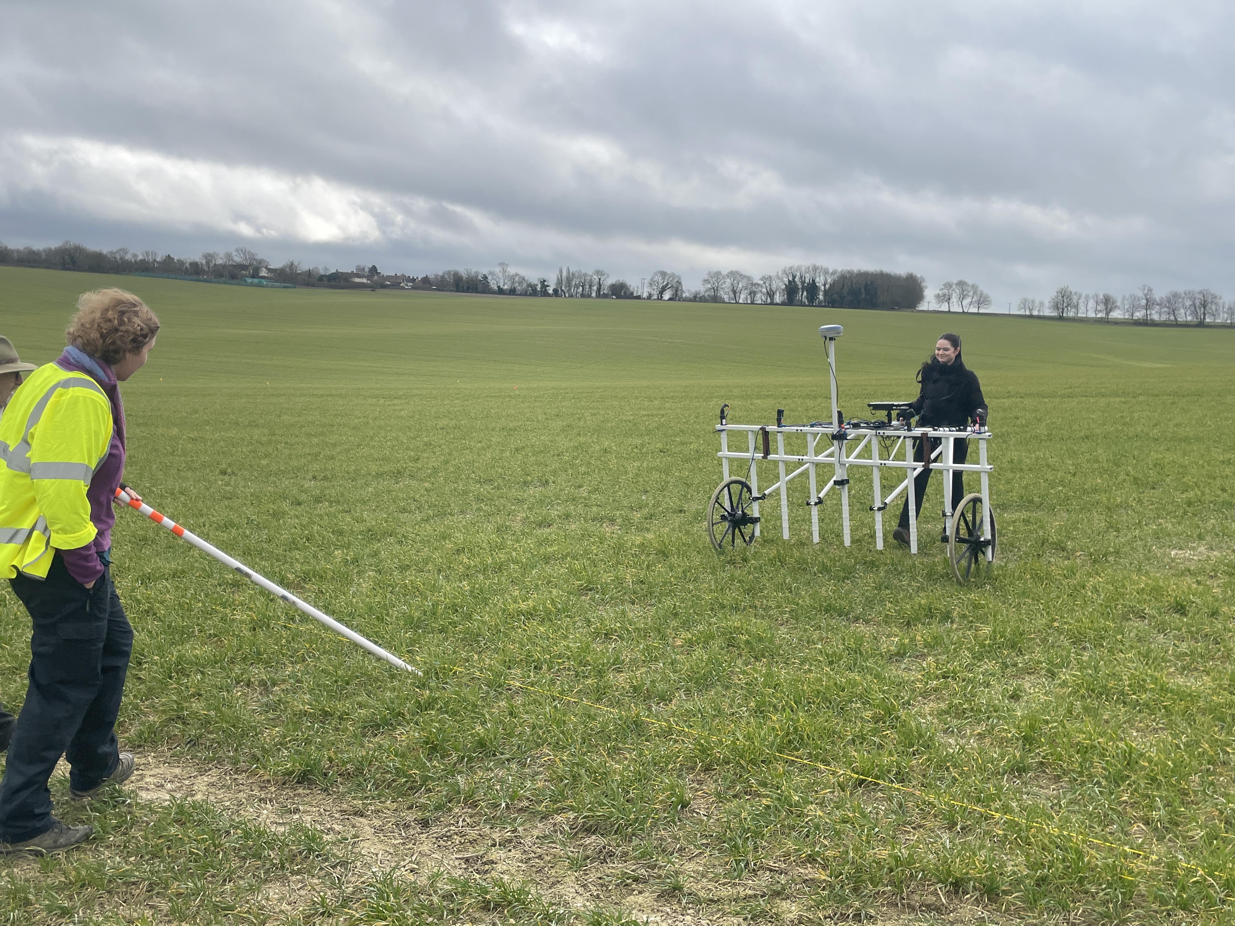
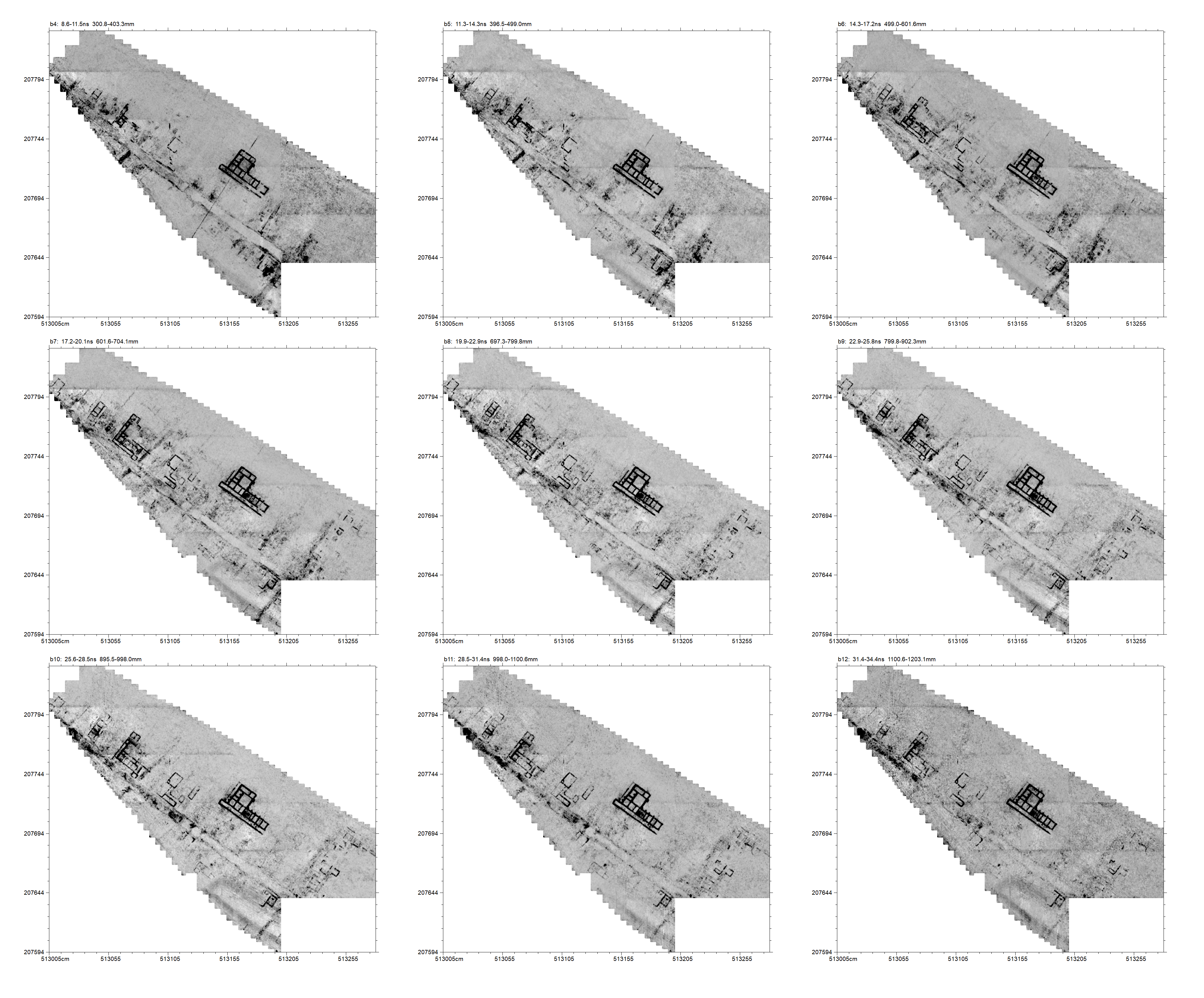
Figure 2 shows the results from the mag survey. Due to the long length of the transect I’ve split it into three parts in Figures 3, 5 and 6.

Figure 2: the whole magnetic survey transect.

Figure 3: the western end of the magnetometry transect.

In Figure 3 we can see two parallel lines running roughly north-south indicated with the red arrows. These were seen in the earlier survey and also in some of the Google Earth imagery. The most likely explanation is they indicate the line of the Roman road. In order to test if there might be buildings either side of the road we did a limited Earth Resistance survey (Fig. 4).

Figure 4: the Earth Resistance survey overlain on the magnetometry survey.

In Figure 4 I have overlain the Earth Resistance survey on the magnetometry. The left-hand image is from the survey with a 0.5m mobile probe separation. That survey is “looking” roughly 50cm below the surface. The two ditches show very well, and higher resistance readings between the ditches at the north end suggest some of the road make-up may survive. The readings decrease to the south and the ditches become less clear. This is probably because we are moving downslope and there is an increase in the depth of colluvium. The 1m probe spacing data on the right is less clear and more dominated by roughly east-west stripes. These are following the cultivation lines. I speculate that these are connected to cultivation, maybe deep ploughing?

Figure 5: the centre section of the mag survey.

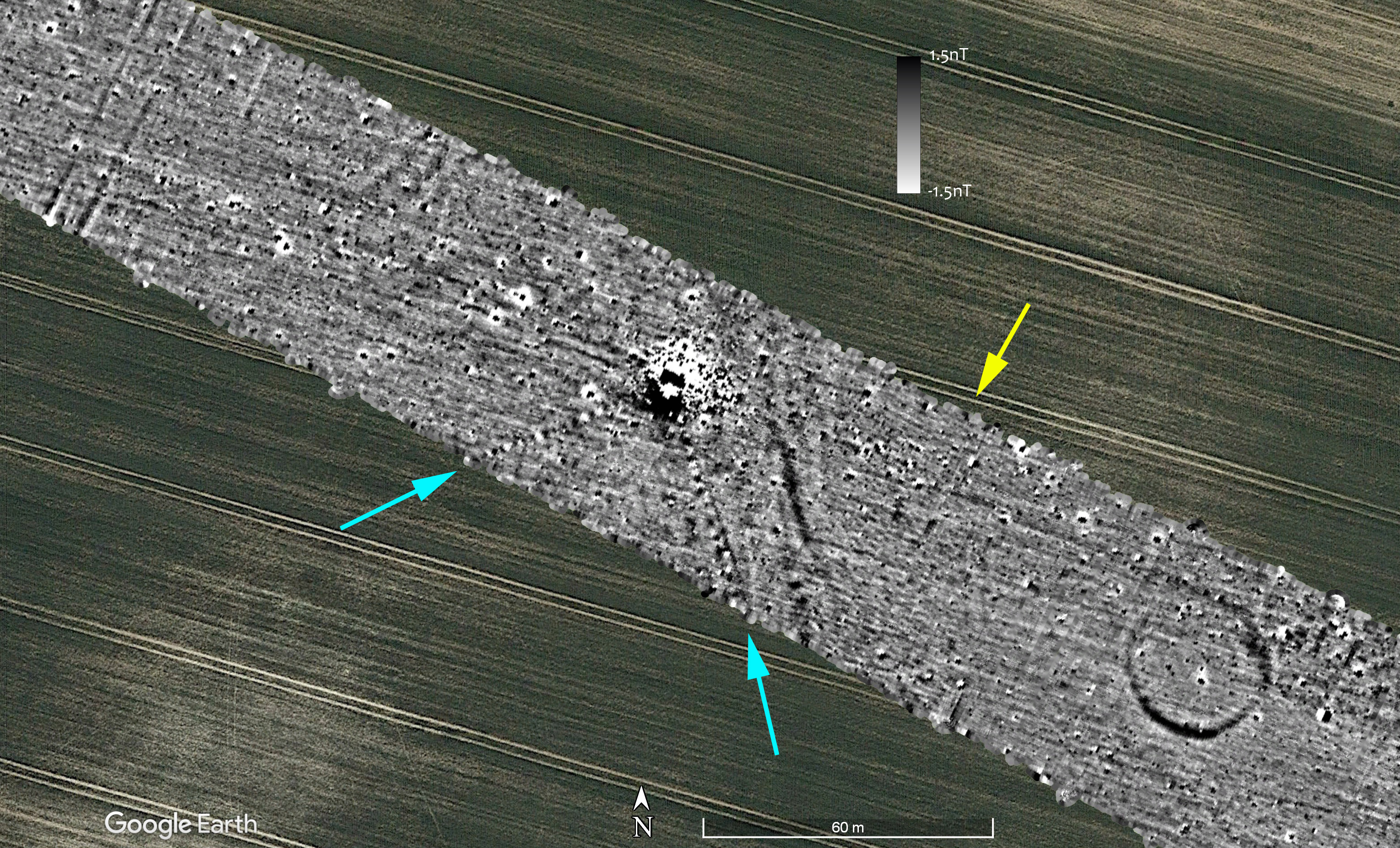
The centre of the survey is less interesting (Fig. 5). The messy black and white blob in the middle is a modern ferrous feature. In some earlier Google Earth images the ploughing goes around it. There are two pipes going towards it (indicated by the blue arrows). The magnetic contrast in this field is very low. I have clipped the image to +/- 1.5nT. For comparison, the Verulamium surveys are often clipped to between +/-6nT and +/-9nT. The very slight “ripple” look in the block indicated by the yellow arrow is due to the operator having something ferrous on them at the time (car keys, wallet, phone in a pocket for example?). Although the cart is much more tolerant of the operator having something magnetic on them (after all, we have a giant battery on our backs!), it is not immune especially when we have to clip the data quite harshly as here.

Figure 6: the eastern end of the mag survey.

At the eastern end the main feature is the ploughed out round barrow indicated by the yellow arrow. The upslope part is less clear probably because it was under a later field boundary that can be seen on the historic maps. The striping seen at the far end indicted by the red arrows are erosion channels in the relatively steep slope here. Just outside the survey area were a series of sand and gravels quarries shown on the historic OS maps.

Figure 7: the Earth Resistance survey over the barrow.

On the second day we had just enough time to survey a single 20x20m Earth Resistance block over the barrow (Figure 7). Unfortunately, my plotting was a little too accurate and the survey was almost exactly inside the line of the barrow! It would be lovely to redo this at some point.

Figure 8: the mag sus survey underway. Kris Lockyear is using the Bartington mag sus meter, Andy Instone (HHER) is recording the location with the GPR and Sarah Talks (CAGG/Ashwell Museum) is using the Mark 1 data logger. Photo: Daniel Phillips.

We were able to take some magnetic susceptibility readings on the second day (Fig. 8). The aim over the long term is to take some readings at the site of most of our mag surveys so we can build-up a data base of values compared to the “success” of the mag surveys as well as contributing to being able to interpret the wider geophysical surveys. Figure 9 shows the results.

Figure 9: the magsus survey.

The mag sus survey shows quite low contrast in readings going from 20 to 50 si units. The higher readings, however, do show the presence of the old field boundary which can be seen in the historic maps and the local relief model derived from the lidar data (Figure 10). The slight surviving bank from the field boundary was not at all obvious when walking around the field.

Figure 10: Local relief model derived from the 1m lidar data using QGIS. Hill-shading is from the SW. Red line: the magnetometer survey area. Red arrows: removed hedge line showing as a slight bank; blue arrows: linear depression; green arrow: small mound at the location of the ferrous magnetic feature. Data is used under the Open Government licence v.3.0. (Data downloaded from https://environment.data.gov.uk/DefraDataDownload/
?Mode=survey on 2023-04-14.)

For more details on this survey, please consult the report linked above. One of the great things about working with CAGG is how it brings together quite mixed groups, in this case members of CAGG, students from UCL and the staff of the Herts HER. Many thanks go to Daniel Phillips for suggesting this survey and helping organise it. The team consisted of: Ruth Halliwell (CAGG), Jim West (CAGG), Graham Spurway (CAGG), Pauline
Hey (CAGG), Sarah Talks (CAGG), Daniel Phillips (HHER), Andy Instone (HHER),
Rebekah Hart (HHER), Greer Dewdney (HHER), Julia Rogers (UCL), Fiona Yuen Lam
Laii (UCL) and Charlotte Trudinger Charnley (UCL). We would also like to thank PACE
Jolt Energy Ltd, for facilitating access to the land.

GPR at Gorhambury 2022

Regular readers of the blog might have been wondering what is happening this year. I can only apologise that I haven’t been able to write my daily update during the 2022 season. I also have a backlog of other sites to write-up which will get posted when I have the chance. In this post I am going to concentrate on the GPR survey. We have some exciting news on the magnetometry front too which I will save for another day.

Last season (see previous posts for August 2021) we surveyed roughly half of the field to the north of the drive at Gorhambury. This field is called “Blackgrounds” although the team usually call it “the macellum field” after the building excavated there in 1938 by Miss K. M. Richardson. We had completed the magnetometry survey of this field in 2016 (Fig. 1).

Figure 1: Magnetometry survey in Blackgrounds.

The magnetometry survey revealed the course of Watling Street very clearly. Some buildings show extremely clearly, and there are many indications of walls seen in the results as white lines. Remembering that something magnetic has a positive and negative pole (north and south if you like), why do walls show as negative? Mid-grey in these figures represents “neutral”, or the average background value for magnetism. Topsoil and archaeological sediments are often more magnetic than subsoil which is why things like the aqueduct show so clearly. A flint wall is not magnetic, but it occupies a space in the slightly more magnetic surrounding deposits, and therefore shows as a negative reading. If you zoom in to the image you can start picking out many walls, and some make clear rooms and buildings.

Last summer we completed about half of this field using Ground Penetrating Radar (GPR). We use the UCL Institute of Archaeology’s Mala GX with a 450mhz antenna. Many thanks to the IoA for allowing the use of this equipment! We mainly collect data in 40x40m grid squares at 0.5m transect intervals. The radar sends a pulse into the ground roughly every 3cm (Figure 2).

Figure 2: Nigel (NHAS / NCAG / WAS) using the GPR.

The GPR results last summer were really nice, but left us hanging as some really fascinating looking features were starting to show (see “A happy ending”). Well, this year’s survey has not disappointed! Up until now, the survey results have been great but mostly we have found the sorts of things one would expect in the town: roads, small buildings, big buildings, pits, kilns and ditches. This season’s results have had us asking “what is THAT building?” Why? Because they are huge and of unexpected forms. Figure 3 shows all the results up to the end of August 24th.

Figure 3: the GPR results up to the end of 24th August 2022.

Figure 3 shows the Insula XXXVII Building 1 very clearly. This building has been long known and can be seen very clearly as a parch mark on Google Earth. The line of the 1955 ditch — the first century boundary of the town which went out of use, according to Frere, in c.125 — doesn’t show very clearly in the GPR data but is important. Why? Well, the buildings to the NW of the ditch (i.e., outside the early town) all look like the sort of domestic / small business properties one would expect and have seen elsewhere in the town. The buildings to the SE of the ditch, and north of Watling Street, have a very different feel to them.

Figure 4: Block 1.

Figure 4 shows what I am going to call for the purposes of this blog post “block 1”. Here, we seem to have traces of some buildings around an open courtyard. The building in the north-east corner looks well preserved, the others are harder to make out (further data processing might help). The southern edge along Watling Street appears empty of buildings apart from one small on in the SE corner.

Figure 5: Block 2.

Figure 5 shows block 2. I have used an “overlay” analysis to try and improve the visibility of the building. On the NE side of the building we have a range 80m long with a 60m colonnade. It has about 20 columns. To give you a sense of scale, the nave of St Albans Abbey is 85m long. The colonnade looks out over the River Ver which runs to the north. The building seems to be subdivided into many smaller rooms. At either end is a projecting wing, the one on the east end having an apse.

Behind this main range there appears to be a corridor, then an open space, and then another very long building. This one has a central protruding room and two wings, but does not seem to have the multitude of internal rooms of the northern range. Behind this is what might be another courtyard with more rooms in the southern corner.

This building begs many questions. Is it all one phase? Are there connecting rooms or corridors (there are hints)? Do some rooms have floors surviving? Some of these questions can, hopefully, be answered with a programme of detailed data analysis: producing more time slices using different parameters and filters as well as looking at the all-important radargrams.

The biggest question is, however, what is this building? I’ve shown the plan to a few people and no-one has come back to me with an unequivocal answer. The word “palace” has been mentioned by several. If it is a “palace”, to whom does it belong? There are definitely more questions than answers at the moment.

Figure 6: Block 3.

Figure 6 shows block 3. Starting from the NE corner, we have faint hints of a road surface which appears to have gone out of use and been built over. Then there is a large structure, again with an apse. This might be an upmarket house? Behind that is the most curious area. There appears to be a courtyard building with rooms on the inside on the southern side, but rooms on the outside on the northern edge. Aligned SW-NE is an aisled building with quite large foundations. This building is roughly 45m long and 16m wide. It is at a slightly different alignment to the buildings in the next block and appears to cut by then suggesting it is earlier and went out of use. In the courtyard, perhaps attached to the aisled building are two large rooms. Further out into the courtyard, and quite deep in the radargrams, is another building only visible as fragments but with large buttresses.

Figure 7: block 4.

Figure 7 shows block 4 which is bounded on its SW side by Watling Street (Niblett and Thompson Street 14) and on its SE by Street 24. Its NW side is bounded by block 3 discussed above and the NE side faces the River Ver. Starting on the SW side, we can see two, probably, buildings facing onto Watling Street. Then behind them there appears to be a series of buildings within another courtyard. It is quite hard to make out what is inside and what is outside, but it certainly appears as a coherent, and almost symmetrical arrangement of rooms and buildings with that area. In the NE corner, just outside “courtyard” is a large single room building some 10m by 13.5m in size. Projecting from this at an odd angle is another feature, maybe a drain? Street 24 is an important road as it heads to the so-called “theatre gate” and there is some evidence of the road crossing the Ver at this point and going into the field opposite, but that is the topic for another blog post.

At the bottom of Figure 7 there is another building on the other side of Street 24. This building is the “macellum” excavated in 1938 which I will discuss in another post.

Surveying at Verulamium has always been very satisfying, and we have got some excellent results since the first season in 2013. The latest results will, however, generate a lot of discussion as to what these buildings are, and what they tell us about this fascinating Roman city.

Many thanks to the team for all their work this year especially Ruth, Pauline, Rhian, Jim, Mike, Nigel, Graeme and John. More updates soon!

A happy ending

Most years two things have happened. Firstly, we have lost two days to bad weather and secondly, we’ve had some little job to finish off on the Bank Holiday. This year, although the dead Foerster mag resulted in us spending the first three days on another site using the Bartington magnetometer instead, and the late hay harvest delayed our start for the Earth Resistance survey in the Theatre Field, we have not lost any days for bad weather and we have met all my targets for the year so will not be back tomorrow. Go team!

Before I get stuck into the results and the usual end-of-season stats, I’d like to say a big thank you to all the team. Twenty people were involved in the work this season, some just for the odd day, some for almost every day. I’d especially like to thank those who helped ferry stuff and look after it over night, who helped fix stuff, and for ferrying me. You all know who you are. All your efforts are really appreciated and the project would not be the same, or even possible, without you. I’d also like to thank Lord Verulam for facilitating access to his land. There are some days when I am high on the hill overlooking the Roman town, with the cathedral on the horizon, that I cannot believe I can be so lucky as to be able to work here each summer.

The Earth Resistance team managed an excellent seven grids today to complete the southern transect to the hedge line (Fig. 1).

Fig. 1: the res team on the last day.

Over the last 17 days at Gorhambury the resistance team have collected data from 75 grids. Since moving into the Theatre Field they have averaged six grids a day. Those 75 grids cover 30,000m² or 3 ha. The team have stabbed the ground with the machine some 60,000 times, collecting 180,000 readings, 120,000 0.5m spacing readings and 60,000 1m spacing readings. The area covered is a bit odd looking because we have been adding to the edges of the area previously surveyed (Fig. 2).

Fig. 2: the 2021 Earth Resistance survey.

The GPR team had a few problems with the new system at the start of the season, but they soon got into the swing of things and have completed 4.12ha of Blacklands Field (Fig. 3). The field is 7.97ha, so they have completed 51% of the field, some 82,400m of radargrams which occupy some 3.14gb of my hard-disk!

Fig. 3: Blacklands Field GPR at the end of the 2021 season.

Despite Fergus’ indifference (Fig. 4), the res team did a great job today. The results are quite subtle (Fig. 5).

Fig. 4: Unimpressed.

Fig 5: the results from the Earth Resistance survey.

Although the results from the survey aren’t hugely obvious, we may have found a couple of buildings. I had indicated them with the res arrows in the image. I’ll have to cross-reference them with the mag and GPR images to be sure.

Figure 6 shows nine time slices from the GPR survey.

Fig. 6: nine time slices for the GPR survey at the end of the 2021 survey.

Today’s survey has revealed a series of buildings on the eastern edge of the survey area. Figs. 7-9 show three time slices in more detail.

Fig. 7: slice 5.

Fig. 8: Slice 9.

Fig. 9: slice 11.

We clearly have a series of buildings around a open area with Watling Street on the SW side. To the east, there appears to be a walled enclosure. Some of the buildings appear to have columns in front, especially the small one in the SE corner. The buildings do not look like the big town houses we have found in much of the rest of the town. I’m going to have to do some research into the plans of other types of building.

We also finished the mag sus survey today, We collected some 1,300 readings which I’ll have to type in. Unlike our other survey methods, the mag sus meter uses a Mark 1 pencil data logger…

I’ll post updates on the data processing, and on some other surveys I haven’t had a chance to write-up over the following weeks. Meanwhile, we’ve pulled-up our last flag at Gorhambury for another year (Fig. 10).

Fig. 10: the last flag.

Just one day more

If you are new to geophysical survey in archaeology, please visit the introductory page “Geophysical survey in archaeology”.

I always have mixed feelings at this time of year. I so enjoy spending the days out in the fields at Gorhambury with the gang, and the end of the season marks, for me, the end of summer and the start of getting ready for the new term. On the other hand, I’ve had, essentially, one day off in a month so I am looking forward to putting my feet up, at least for a day!

We ran all three machines today: the Earth Resistance Meter, the GPR and the magnetic susceptibility meter. All three managed a good area and hopefully we’ll all meet our targets by the end of tomorrow so we can avoid the traditional extra part-day on the Bank Holiday. The mag sus has now taken well over 1100 readings, but I’ll make a separate posting about that in due course.

Fig. 1: Gill, Pauline and the resistance meter, watched by Fergus.

The Earth Resistance team are a very long way from the rest of us, at the top of the hill overlooking the town. They are working eastwards towards Bluehouse Hill.

Fig. 2: the Earth Resistance survey after day 16.

The survey (Fig. 2) shows the 1955 ditch and the buildings I mentioned yesterday. There is quite a contrast between some areas on the edge of the dry valley and the buildings making them harder to see. With a bit of careful data processing I can, hopefully, bring them out more clearly.

The GPR survey’s two 40x40m blocks had one or two buildings in them. Fig. 3 shows time slice 9.

Fig. 3: GPR slice 9.

We seem to be in an area of public buildings and open spaces, rather than private houses like the “motorway services” (which I think is actually a very nice house and not services at all!). We are going to be left with very tantalising half-surveyed buildings until next summer (we hope).

Short posting tonight as it is getting late and tomorrow is our last day.

Chilly

For those unfamiliar with geophysical survey techniques in archaeology, please visit the “geophysical survey in archaeology” page for an introduction.

I know it is getting towards the end of August and the nights are drawing in, but who turned the heat off? It was really rather chilly out on site today, and the wind didn’t help.

The magnetic susceptibility survey continued today thanks to the help of Gill and Julia. At my request, Julia came in today specifically to help with the survey, so many thanks. The survey technique is a peculiar mixture of high and low tech. The mag sus meter itself looks like a thirty-year-old design, and probably is! It has no data logger or GPS. The survey method, therefore, is as follows:

1. Hold the loop of the meter high in the air and hit zero.
2. Hold the loop of the meter as flat on the ground as possible and hit measure.
3. Shout out the reading and the second person writes it down in the notebook.
4. Take a GPS measurement where the reading was taken.
5. Pace out roughly five meters to the next point and repeat.

The easiest way to do this is with three people (Fig. 1).

Fig 1: the mag sus survey in action (photo: Mike Smith).

I haven’t had a chance to type in the 892 readings we have taken so far to process them, but I have downloaded the coordinates to see how well our system of pacing out distances towards a ranging rod is working. There are a few gaps, but not too bad (Fig. 2)!

Fig. 2: the location of the magnetic susceptibility readings.

The GPR team spent the day in doing the saw tooth southern edge of the Blacklands field. The lines started quite short, but ended-up at 52m. Not that much longer than 40m, really… (Fig. 3).

Fig. 3: collecting long GPR transects (photo: Mike Smith).

The buildings on the edge of the GPR survey yesterday continued to show-up very nicely. Figures 4, 5 and 6 show slices 5, 9 and 11. Remember that the higher slice numbers are the deeper ones.

Fig 4: GPR slice 5 after Day 15.

Fig. 5: GPR Slice 9.

Fig. 6: GPR Slice 11.

The strong (dark) response across Watling Street seen most clearly in Slice 5, and as more of a blob in slices 9 and 11 is the northern triumphal arch excavated in 1961 by Frere. It had been seen in an aerial photograph by Dr J. K. S. St Joseph.

Many of these buildings do not seem to appear in Alban’s Buried Towns but we have seen some of them before. Fig. 7 shows the magnetic gradiometer data from 2016 in the same area.

Fig. 7: the mag data in the same area.

The mag and GPR together do seem to suggest that there is a large open space here, with buildings along the sides, especially to the south of Watling Street. Lots of things to speculate about!

The res team completed another six grids to hit the target I set them a while ago two days early (Fig. 8).

Fig. 8: the complete res survey with the mag survey in the background.

Figure 9 zooms in on the southern area to show the grids collected recently.

Fig. 9: the southern edge of the res survey.

The latest blocks have picked-up the 1955 ditch (as seen a bit more clearly in the mag data) and interestingly, a road which runs behind the ditch. It has also completed some buildings that were surveyed in earlier seasons. The team now have a bonus prize (!) of completing a line of 12 grid squares along the southern edge of the survey, ending-up at the side of the road up Bluehouse Hill. To encourage the team, some nice buildings can be seen in the magnetic data!

Those of you who have followed this blog over the years may be surprised that I haven’t used one of my favourite words, as is traditional on the last Friday of the season. Well, I decided using antepenultimate was getting a bit old… oops. I just used it again. Oh well…

A bit busy

If you are new to geophysical survey in archaeology, please visit the “Geophysical survey in archaeology” page.

It seemed as though today was quite busy. There are times when I wish I could clone myself, or at least we had two dGPS units! It wasn’t helped by leaving the all important “brown bag” at home with my notebooks, so big thanks to Ellen for bringing it over. Both teams completed excellent areas, two 40×40 grids for the GPS and six 20x20m grids for the Earth Resistance. Pauline, Georgina and I also completed some more magnetic susceptibility survey despite a large haystack in the way. I think Thistle (Fergus, CAGG’s watchdog’s best friend) thought we were utterly mad dragging her back and forth across the same bit of field.

The res team is still heading south, although they only have six grids left to complete the transect I hoped they would complete (Fig. 1).

Fig. 1: The Earth Resistance survey to date.

With luck the team will complete the last six grids tomorrow and then what will they do on the weekend? (At this point imagine an evil Mutley-like laugh…) Yes, I have an idea…

Fig. 2 shows a detail of the southern end of the transect the team have been working on.

Fig. 2: detail of the survey. The darker strip to the west is the 2021 survey.

As you can see, the survey picked-up the southern end of the buildings, but has gone back into an area of nothingness. What is not visible in the image is that there is an undulation in the field surface, and the diagonal SW-NE area of blankness south of the hedge is a slight dry valley. The question arises, therefore, is the “blank” area actually empty, or can we not see the archaeology due to the build-up of colluvium? We may get the answer from Oxford Archaeology’s test pits excavated in 2000 (Fig. 3).

Fig. 3: Oxford Archaeology’s test pits from 2000.

At 10pm after a busy day I’m not going to start looking at that data now, but it is obviously quite important. Verulamium Museum also has a large box of 35mm slides from the test pitting exercise, if someone fancies a job scanning them…

The GPR team had a slight problem at the start of the day when one of their antenna batteries had not charged properly overnight. Thankfully, the second battery lasted the rest of the day… just! Here are the usual nine time slices (Fig. 4).

Fig. 4: Nine time slices from the survey up to the end of day 14.

Today’s survey revealed a mass of buildings to the south of Watling Street. It looks like the buildings to the north of Watling Street might be arranged around a large open area. Cutting across Watling Street is a curiously strong response, some sort of quite substantial foundation. Is this just a spot where the robbers missed a section of road, or something else? Figs. 5-7 show three slices of increasing depth so that you can see how this changes as we go deeper.

Fig. 5: Day 14, time slice 4.

Fig. 6: Time slice 9.

Fig. 7: Time slice 11.

I spent the last hour of the day laying out the “saw tooth” edge to the field ready for the team to survey today. Given the buildings going into that area, it should be an exciting set of data tomorrow.

A glorious day

The weather today was lovely and reminded me of how much I love working in the Theatre Field. Although the hill leaves one a little breathless (especially when carting gear up it) the view across to the abbey is just lovely (Fig. 1).

Fig. 1: St Albans abbey in the sunshine.

Many thanks to Mia, Gill and Georgina for helping me with the magnetic susceptibility survey. No results to show as yet (I have to type them in!) but we did cover an area 140m x 60m at roughly 5m intervals, about a third of the area I’d like to get done this summer. Hopefully, this survey will help us understand why some buildings show in the magnetic survey data, and some do not.

The GPR crew had a screw loose this morning. No, I mean an actual screw. Well, probably is it technically a bolt. I looked down from the hill to see them scouring the grass. Thankfully, we had another bolt which sort of fitted and allowed them to carry on and complete another 80x40m block. Fig. 2 shows the time slices.

Fig. 2: nine time slices from the survey up to the end of day 13.

They found lots of bits of buildings, but it looks like whatever was here has been a bit more robbed out than some of the other buildings we have seen. For a change, Fig, 13 shows time slice 13.

Fig. 3: time slice 11.

The building parallel to the wall at the northern edge of the survey area, towards the eastern side, appears to have a large apsidal room. This looks like the sort of dining room we get in the fourth century such as the one at Lullingstone villa. Traditional Roman dining rooms had three couches arranged around three sides of a square, hence triclinium. In the fourth century the fashion changed to have a U- or omega-shaped couch, and hence the dining rooms became apsidal.

The Earth Resistance team completed an excellent six grids, although one had to be in two parts as it straddled the hedge line. Sadly, there wasn’t much in it (Fig. 4).

Fig. 4: the Earth Resistance survey. Today’s grids are the slightly darker block to the west.

OK. I lied. The grids are stuffed full of buildings with Street 25 running right through the middle. Bits of these buildings could be seen in aerial photographs from 1976, but with nothing like the clarity we see here. These are super results.

Tomorrow sees us back on site as the end of the season rapidly approaches. Hopefully, I’ll get a bit more mag sus done, and the other teams will continue their excellent progress.

Two hundred

Two hundred what?, I hear you ask. Well, this is the 200th posting to the hertsgeosurvey blog. Who knew I could be so verbose? Well, generations of Institute of Archaeology students probably have [impolite] opinions on that!

In the morning, Mike, Nigel and I worked with the GPR. Normally, I’m off with my “staff of position” as Peter would call it, but GPR with only two people is not fun, especially in the long grass. Many thanks to Sonia for turning out this afternoon to help move strings having only got back from holiday yesterday. It was most appreciated. The GPR completed two 40x40m blocks, the second with “saw teeth” along the northern edge. Fig. 1 shows nine time slices of the whole survey area.

Fig. 1: nine time slices of the whole survey area.

Figure 2 shows my favourite slice, No. 9, in context.

Fig. 2: time slice 9 at the end of week 3.

Unusually, the GPR has found traces of a building near the northern edge of the town. So far, the area behind where we think the wall would be has been pretty empty. Fig. 3 shows this in a little more detail.

Fig. 3: detail of the area surveyed this weekend.

There are some tantalising faint marks as well as the more obvious walls, which might represent robbed walls. I’m not entirely sure, but I think this area is just marked as “area of occupation” in Niblett and Thompson (Alban’s Buried Towns). Even more tantalising are the parch marks which can be seen in the unsurveyed area to the south. Comparison to the mag data shows (Fig. 4) that the walls sort of show if you know where they are and squint, but you might not put much faith in them without the GPR. Multi-instrument survey rocks.

Fig. 4: The mag survey for the same area as Figure 3. The red line indicates the edge of the GPR survey.

The weather today was, at times, a bit wet (especially immediately after lunch) but at times was very pleasant (Fig. 5). The very definition of changeable!

Fig. 5: ominous clouds (image © Mike Smith).

The Earth Resistance team completed an excellent eight grids, making-up for my errors of yesterday. Fig. 6 shows the entire res survey on the Gorhambury side of the town.

Fig. 6: the Gorhambury Earth Resistance survey.

The survey is now an impressive 11.5ha which is pretty good going for a twin-probe Earth Resistance survey. At the end of the season I will add the new blocks into the master composite which should get rid of the difference between the old and new parts of the survey in the Theatre Field. Fig. 7 shows a detail of the new area.

Fig. 7: the area surveyed recently (to the west) and adjacent blocks from the master survey.

The diagonal line running NW-SE across the plot is Street 11. It has been robbed to the east of the cross-roads, but appears to be pretty much intact to the west. Although subtle, there are clear buildings in the new area, one just south of Street 11 on the western edge of the survey, and one disappearing into the hedge on the southern edge of the new area. Street 25 can be seen running NE-SW and appearing as a parch-mark south of the hedgerow. There are also clear parch-marks of buildings just off that street which are right in our transect. Exciting prospects for next week’s survey. At the end of week three we finally headed down the hill to the cars (Fig. 8).

Fig. 8: Home from the Hill. (Image © Mike Smith).

Now for a well earned two days off. I’ll be spending them going to Sussex to teach… umm… geophysics. Oh well, no rest for the wicked. Look out for a special bonus post tomorrow.

A bit damp

Today started badly. Somehow I had managed to leave the Earth Resistance meter on and the batteries were flatter than the proverbial pancake, and the weather in the morning was miserable. It was the sort of rain that was light enough that one thought soldiering on was OK, but heavy enough that everything was a bit damp by lunchtime. During lunch the weather dried-up, and apart from one short shower in the afternoon it was not too bad in the afternoon, although the team might not agree with me!

Despite the problems, the res team completed four grids before the dry-cell batteries gave out. They don’t last long. The results of the Earth Resistance survey are shown in Fig. 1.

Fig. 1: The Earth Resistance survey. The strip to the west is the 2021 results so far.

Sadly, the grids are mostly the same odd “noise” as yesterday’s data, although the SW corner clips Street 11 shown as the black (high resistance) triangle in the corner. There is also a large roughly circular feature which shows in the res data and the mag data as shown in Fig. 2.

Fig. 2: the blob (outlined in red) in the res (left) and magnetic data (right).

I have no idea what it is, but it is big (some 9m across, roughly). Some form of burnt surface, maybe?

From the top of the hill where the res team are working, the GPR team in Blacklands Field seem a long way away. Fig. 3 shows the GPR team at work, and this image was taken with a telephoto lens!

Fig. 3: the GPR team in Blacklands Field.

The GPR completed the “saw teeth” on the southern edge of the transect, and started the new transect by surveying yet more saw teeth on the northern edge! Fig. 4 shows nine time slices.

Fig. 4: GPR time slices for days 1 to 11.

Processing the GPR data in one go has some advantages, and some disadvantages. Despite having a fairly powerful computer, it takes a while now to process the whole survey. I also deleted some 30gb of duplicate files this evening. The software makes many copies of the data as it works. Fig. 5 shows my favourite slice, No. 9.

Fig. 5: GPR slice 9.

The completed saw-tooth section on the southern side of the survey area has revealed a nice small building, albeit with its western wall missing. There are also traces of Street 26 running SW-NE. The new transect has started like most of the data close to the line of the wall, with nothing showing. Although we presume the steep bank down to the flood plain of the river represents the line of the wall, we have yet to find anyone mentioning any actual evidence of it.

For people who “know” GPR, you may be wondering why I just say “slice 9” rather than give actual depths. “Slice 9” is pretty meaningless as it depends on the settings one uses in the software (for the 2021 season I have kept these the same). To calculate the actual depths, one needs to know the speed that the radar waves are travelling through the soil. To calculate this, one uses the software to find hyperbolic curves in the data, and then match them on-screen which will give you the speed. The only problem is that the software I use assumes your mouse has a central scroll wheel. Mine does not — I use a trackball. The alternative method involves clicking the mouse, but the curve changes so fast that it is almost impossible to get a match. I’ve given-up for now.

After the hay was baled, the local red kites come to look for dead things in the grass. I get a bit worried when they circle over the team… I’m not really a wildlife photographer, and I don’t really have a long enough lens, but I had a go this lunchtime (Fig. 6).

Fig, 6: a red kite looking for lunch.

Hopefully tomorrow will be a more straightforward day.

A good day

After yesterday’s equipment failure, the GPR team completed their (more usual) two blocks, and the res team six grids, so all-in-all an excellent day. For a change, I didn’t have to do too much flagging-out today (Fig. 1).

Fig. 1: laying-out grids for the Earth Resistance survey.

Seeing that photo does make me realise I need a haircut! The saw teeth edges of GPR grids take a lot of extra pegs (Fig. 2). A normal grid takes four pegs to lay-out, a grid with “saw teeth” along one edge takes 18… Zzzzzz…

Fig. 2: “saw teeth” along the edge of Gorhambury drive. Note the fortuitous inclusion of geese.

The Earth Resistance team are slowly working their way south and up the hill (Fig. 3).

Fig. 3: the Earth Resistance team on the horizon.

Figure 4 shows today’s Earth Resistance results next to those from 2016-2019. The fact that this year’s are slightly darker is a result of the processing (which I left to make it clear which was which) — they have just been plotted side-by-side in Google Earth. Sadly, given the slope we were working up, not a great deal showed in today’s data.

Fig. 4: The Earth Resistance survey in the Theatre Field. The darker band to the west is this year’s data. The lack of match is just due to processing.

There is one linear feature and a great deal of “noise” similar to that seen in previous years in this area. Is this because there were no structures here, or because they have been ploughed away? Within the next block of six grid squares, however, the survey will cross Street 11 which we know from the mag and GPR surveys has buildings along it. Tomorrow’s data should be more interesting.

The GPR team re-did the block that suffered from the problem with the odometer, and then another block to the south (Fig. 5).

Fig. 5: the GPR team of Mike, John and Nick working in Blacklands Field.

Figure 6 shows the whole area surveyed in 2021 (slice 7). As can be seen, it is very busy.

Fig. 6: the GPR survey after day 10 (slice 7).

One question that I ask myself each time I look at this area is why the “motorway services” (aka Monument 302, or Insula XXXVII, Building 1) shows so well in the mag, res, and GPR data as well as in multiple aerial images including those most recently posted on Google Earth from 2020. Is it so fantastically well-preserved?

In Figure 7 I zoom in a little on the area surveyed today. We already know about Monument 302, but the GPR data is revealing more buildings along the heavily robbed-out Watling Street. Tomorrow’s saw-tooth to the south should show more of the building on the edge of the survey area.

Fig. 7: the GPR survey after day 10, slice 9.

There are thunderstorms promised tomorrow afternoon but St Albans is right on the edge of the area predicted. Let’s hope they pass to the west.