Processing mag data (Part 1)

I thought it would be useful to outline how I have processed the magnetometry data from our surveys.

The first stage is to download the data from the Foerster datalogger.  I use their simple and free program IFR Dataload to do this.  Foerster sell a more complex program for processing data from the Ferex, but I find TerraSurveyor easier to use, as well as having the convenience of being able to process data from the resistance meters and other magnetometers.  When I download the files, you can give them a suffix, and they are numbered in sequence.  Usually I use some like “gorday4_” standing for Gorhambury survey, day four. I then end up with a sequence of files: gorday4_1.fdl, gorday4_2.fdl and so on.  FDL is Foerster’s own file format. You can look at each square in Dataload.

Screen grab from Dataload (best seen full size).

Although one can play around with the image at this point, there is no reason to.  If the square is a partial, it is worth making a note of its dimensions.  Each grid square is then exported as a “Text table” which is a fairly simple ASCII file.  I just number each text file sequentially, e.g., gor001.txt, gor002.txt and so on.  If I know that two or more text files are eventually going to be combined into one grid in TerraSurveyor, e.g., when we have surveyed a partial grid square in bits, I use gor003a.txt, gor003b.txt and so on.  You can see the importance of keeping good field notes or processing the data very soon after the day’s survey.

The next stage is to import the text files into TerraSurveyor.  If it is a new site, we need to create it.

Creating a new site in TerraSurveyor.

Having created the new site, we have to import the Foerster text files.  First click on the import button.

The download button is TS.

This will make the import window pop-up. A Foerster template is not currently part of the default installation, you’ll need to get it from David Wilbourn or myself. Once you have it, just select it from the list.

Selecting the Foerster text table import template.

In the next screen, you need to navigate to where you saved the text files exported from dataload and then choose which ones you want to import.  On the first day it will be all of them, but subsequently just the grids since the last time you processed the data.  After that, just keep clicking next and accept all the defaults until the data is imported. The TS grid files will take the name of the text files, so gor001.txt becomes gor001.xgd.

Choosing text files to import.

The next stage is to assemble the grid into a composite.  Either click on “Assemble grids” to create a new composite, or select the existing one and click on “Open Grid Assembly” (all in the navigation window).

Grid assembly (part 1).

In the Grid Assembly window you can see thumbnails of the individual grids.  These can be drag-and-dropped into the grid in the correct pattern.  The direction of first traverse is always from left to right, so if we are surveying south-to-north on the first line of the grid, north will be to the right.  To make the grid bigger, use the blue arrows on the right.

Grid assembly (part 2).

Having completed adding the grids, click on Save or Save As.

Grid assembly (part 3).

At first, the composite just looks uniform gray.

First look at a new composite.

This is because the extreme values from pieces of iron in the ground are being plotted as black and white.  The majority of the values which are much closer to zero are squeezed into a small number of mid-grays.  To see the pattern in the majority of the data, we need to clip the display.

Clipping the display values.

The clip button on the processes toolbar on the left is indicated above.  You can see from the graph in the pop-up window how the values are compressed.  I have entered values of -9 and 9 for the clipping.  Depending on the site, you may need to clip down to as far as +/- 1.5nT.

In the image above I have cheated a bit as the composite has already been clipped.  You can see the archaeology, but the image is very stripy.  This is caused by the sensors being imperfectly compensated, by walking in zig-zags, and by sensor drift.  It is perfectly normal in mag data and can be removed using the destripe command in TS.  Most processing packages call this zero mean traverse as the process alters each traverse (a line of data within a grid square) so that its mean is zero.  TS offers ZMT, but also zero median traverse which is often more robust.  TS, therefore, bundles all the options in the destripe window.

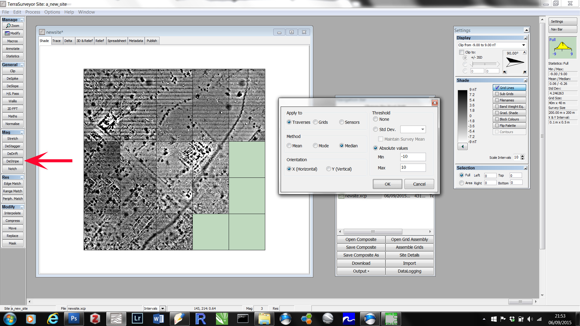
Zero median traverse.

I have indicated the position of the destripe button in the above image.  Often, just accepting the default values is fine but sometimes large numbers of large values can mess this up, and so I set absolute values for the process.  In this case I have used +/- 10nT.

Destriped and clipped.

The resulting image is rather flat.  This is because we have performed the processes in the wrong order.  We should only clip the final image, not the data on which other processes are working.  I did this in the wrong order so that you can see what was happening at each stage, and also to demonstrate the Modify command.  TS, very sensibly, does not alter the base values.  This allows us to edit the processes via the Modify command indicated above.

Modifying and re-ordering processes.

In this case we just want to move the destriping command down to below the clipping command.  Clipping should always be the last command.

Interpolating data values.

The resulting image is pretty good and for quite a while that is all I would do.  Jarrod, however, persuaded that better images could be obtained by interpolation and smoothing.

Interpolating data values.

The first step is to interpolate some new values.  The Foerster collects readings 10cm apart along the traverse, and the traverses are 50cm apart.  This is a rather unbalanced grid.  The traverses are the y-axis in TS and so by selecting the Interpolate button (shown above) and choosing to double the values on the y-axis, we create a grid which is now 25cm by 10cm.

Applying a low pass filter.

The next stage is to smooth the data a little. Obviously, we don’t want to smooth the data so much we get rid of the archaeology! We use a low pass filter.  Click on the button indicated above and select low pass in the window.  I use values of x=7 and y=3.  This is because x=7 is 70cm and y=3 is now 75cm, i.e., close to the ideal of a circular “window” for the filter.

The resulting image will look rubbish.  This is because the processes are again in the wrong order.  Using the modify command, the processes should be in the following order (from bottom to top!)

1. Destripe
2. Interpolate
3. Low pass filter
4. Clip

I have done things a bit backwards so that you can see the effect of each stage.  Normally, I would just do everything in the right order from the start.  If you are adding new squares to an existing composite, the processes will be automatically applied when you save it at the grid assembly stage.  Normally one would only do all this once a survey.

In the next posting I will explain how I deal with partial grid squares.

Apologies to anyone who looked at this soon after I posted it as something went wrong and all the work I did this morning vanished.  I had to re-write half of it again!